By choosing “Users Experiment”, the scan tool will:
Ask you to provide the proposal number.
Validate whether the provided proposal number is correct and valid for this beam time.
If the validation result is okay, the tool will import the proposal metadata and include them in the experimental file. If not, user will be alerted and the tool will not be able to continue!!
Note
The scanning tool is already integrated with the users database. All validation and metadata importing processes are done through such integration. metadata of a validated proposal includes but not limited to proposal title, principal investigator information, number of allocated shifts, proposal review committee.
Choose Local Experiment to run in-house experiment that is not associated with a proposal.
This scan mode is intended to run “not proposal based” experiments, example of such experiments:
Director general beamtime
In-house research experiment
Testing / commissioning new components at the Beamline
Warning
Normally, this option is restricted to beamline scientists.
Warning
Access to experimental data generated out of this kind of experiment is restricted to beamline scientists and authorized SESAME staff only. On the other hand, the generated data will not be mapped/linked with any proposal or PI work.
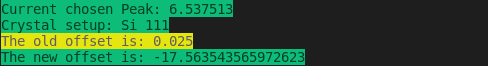
Choose Energy Calibration to calibrate the beam energy in reference to the DCM crystal and metal foil you are using.
The beam energy is linked to the monochromator via the Bragg formula, calibrating the energy means adjusting the Bragg angle (Θ theta) of the monochromator in reference to the crystal and the metal foil you are using.
Currently, the following crystals are available:
Si(111)
Si(311)
Also, the following metal foils:
Ti (4966)
V (5465))
Cr (5989)
Mn (6539)
Fe (7112)
Co (7709)
Ni (8333)
Cu (8979)
Zn (9659)
Se (12658)
Zr (17998)
Nb (18986)
Mo (20000)
Pd (24350)
Ag (25514)
Sn (29200)
Sb (30491)
Ta (9881)
Pt (11564)
Au (11919)
Pb (13035)
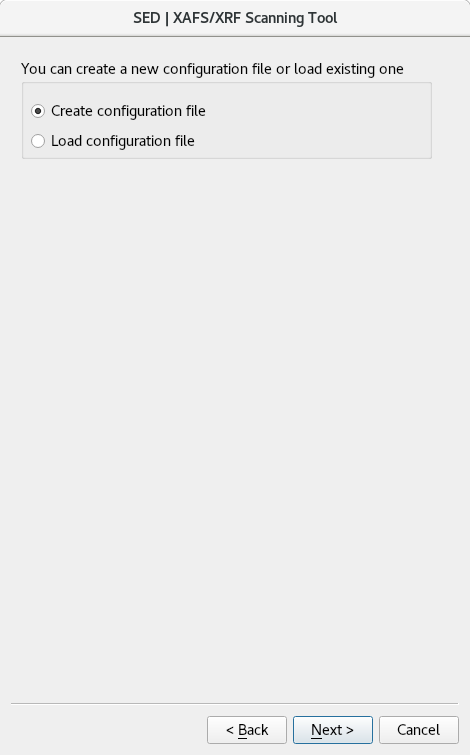
The scanning tool allows you to either enter new configuration and thus generate a new configuration file or load an already existed configuration file. These two options can be chosen from this GUI:
Figure 3: configration mode choosing GUI, either to create new config file or load already existed one
Next GUI is meant to enter new experiment configurations or see/edit a loaded one. This GUI allows you to move the energy over a range by driving the theta motor of the Double Crystal Monochromator (DCM).
The user can enter many intervals, each interval has start energy(eV), end energy(eV), energy move step size, Ionization Chamber (IC) integration time, fluorescence detector integration time, external trigger and step unit.
The step unit can be either in eV or K. When eV is chosen, the “step” is used as energy incerment value across the interval starting from “start” until reaching the “end” energies. By choosing K as step unit, the energy increase size (step size) increases as the scan moves further above the edge.
Note
“The XAFS region is most naturally thought of as a function of k. Because E is proportional to the square of K, features will tend to broaden and reduce in amplitude as getting further above the edge. In addition, the signal falls off with increasing energy, further reducing the amplitude of features high above the edge.”” reference: XAFS for every one, page 161, point# 3
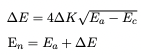
The equations of calulating DCM energy with K step unit are shown below:
Where ΔK is energy step size in K, Ea is the current DCM energy in K, Ec is the calibrated energy in K and En is the next energy value that the DCM is going to.
You can define many samples and align them with respect to the beam (depending on the number of holders installed on the sample stage). Through this GUI you can change the sample position horizontally and vertically in order to target the right position of the sample. Also, for each sample you must assign name where it will be used as part of the experimental file name.
sample name is added as part of the experimental file name
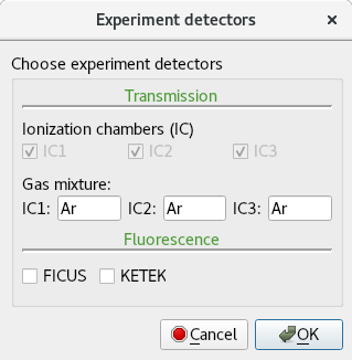
Detectors GUI allows you to choose among the available transmission and florescence detectors. ICs detectors are already chosen by default, you just need to enter the gas mixture that you use in each IC. For the fluorescence detectors, either FICUS or KETEK. For more information about the detectors, please see this page: https://www.sesame.org.jo/beamlines/xafs-xrf#tabs-7
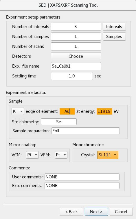
Other scan parameters in the main confirmation GUI like “Experiment metadata”, “Mirror coating” and “Comments” sub-boxes are used to provide some experimental meta data.
Note
Some experiment metadata fields are mandatory because they are needed to comply with xdi file format.
Fields that are highlighted in green (refer to Figure 4) are write protected when you run Users Experiment or Local Experiment (refer to Figure 1). This means that the DCM has been already calibrated and has got these values in which can’t be changed for this kind of experiments.
However, to re-calibrate the DCM with different metal foil element and crystal you can choose Energy Calibration (refer to Figure 1), then, such fields are not “write protected” and you will see them highlighted in orange:
Figure 9: Main configration GUI that belongs to DCM energy calibration
By clicking “Next”, if all is fine, the last GUI will pop up as shown below:
Figure 10: Last GUI before triggering the scan to start
Once scan is started, interactive logs will be printed on the terminal showing exactly what is being processed. Also, an interactive data visualization tool will start plotting the experimental data.
If the Confirm button is clicked without choosing a value, an error messages will be shown in the terminal.
Note
To ignore the smoothing filter, both smoothing parameters in the GUI should be zeros.
Note
To repeat the energy calibration process without running a scan (or when you already have a calibration xdi file), type the following command in terminal: